Questi Appunti semi-(dis)ordinati di Matematica per il Liceo (e forse qualcosa in più) vorrebbero riassumere, molto sommariamente e senza la pretesa di sostituirsi al libro di testo, quanto necessario per affrontare dignitosamente la prova scritta di matematica all'esame di stato. Inoltre, potrebbero risultare utili anche agli studenti iscritti al primo anno di facoltà scientifiche. Per loro natura sono e saranno in continuo divenire; di conseguenza questa pagina verrà costantemente aggiornata. Chiunque scovasse degli errori o avesse dei suggerimenti è vivamente pregato di contattarmi.
Equazioni e disequazioni: principi di equivalenza, intere di primo grado, fratte, intere di secondo grado, intere di grado superiore al secondo, sistemi, irrazionali, con valore assoluto, logaritmiche, esponenziali, goniometriche.
Funzioni: definizioni preliminari, grafico di una funzione e sue caratteristiche, funzioni elementari, operazioni algebriche e di composizione, dominio, grafico di una funzione dal grafico di un'altra.
Limiti: il concetto di limite, la sua definizione e la sua verifica, limiti delle funzioni elementari, algebra e calcolo dei limiti, risoluzione delle forme indeterminate, limiti notevoli.
TopNel secolo (e millennio) scorso, insieme a Marco Caliari, ci impegnammo a raccogliere quanto sapevamo (allora) per aiutare gli studenti di liceo scientifico a superare la seconda prova di maturità. Ne vennero fuori questi appunti di matematica che ho di recente ritrovato e scansionato: prefazione e indice, disequazioni di vario tipo, studio di funzione e integrali
TopThe general purpose of this page is to share some useful programming tips with whomever might be interested.
I am definitely a bad programmer. However, in the last few years I have experienced a tremendous need to systematically organize the scripts that I normally use for work so as to be albe to run an old program right away without wondering for hours what it does (comments are really important!!!). As you will soon realize, I prefer the shell programming to the use of more sophisticated interpreters (Perl, Python, etc.), simply because basic UNIX commands are available on any Linux/UNIX platform.
If while going through these programs (scripts) you discover bugs or find better and more efficient ways to do the same things (I am sure there is plenty!), please let me know.
TopThese are some Octave scripts (compatibility with Matlab was not checked) that I wrote for teaching purpose, avoiding as many loops as I could so as to to make the scripts efficient.
lbvp3x3.m: solves a linear system of 3 ODEs in 3 unknowns with mixed boundary conditions on a generally uneven grid.
blasius.m: solves Blasius equation for the incompressible boundary layer past a flat plate on an uneven grid. Requires vector of independent variable η at grid nodes and returns stream-wise and normal-wall velocity components U(η) and V(η).
TopDo you love Gnuplot but find Octave not as flexible as you would like for making highly-customized (mainly postscript) figures? Then you are definitely the person this script was meant for!
TopIf you use extensively Octave and Gnuplot you might agree with me that the former is a great environment to run computations but sometimes it looks not very flexible to people that use the latter for making highly-customized figures, i.e. figures with special labels, arrows, mathematical formulae in the legend or on the axis, and so on. A simple example is, from version 3.0.0 of Octave, the impossibility to make plots with bullets (or filled circles), available in previous versions of Octave.
gps (GnuPlot Stream) is intended to be called from Octave to generate two-dimensional and three-dimensional plots using the data from Octave and a stream of Gnuplot commands sent to an X11 window. Therefore, all gnuplot features are usable, including the possibility to plot both data from Octave and data saved on disk. The only drawback (at least so far) is that data passed from Octave to gps are written on local (hidden) files. This is necessary to allow the full usage of 'replot'. It should be mentioned that Octave provides low-level Gnuplot commands which, apparentely, should do the same as gps. However, the name of these functions change with the version and it looks like they will be removed from future versions of Octave.
Some pieces of Octave code employing gps and the corresponding figures are reported below.
TopDownload gps.m and save it either in your working directory or in the Octave directory that contains the plotting functions (normally /usr/share/octave/X.Y.Z/m/plot/, where X.Y.Z is your version). You can also save it wherever you prefer and add that path to Octave. Once you have gps.m, have a look at its help from Octave (type help gps). I suggest you download demogps.m and run it to have an idea of what gps can do. You need to make sure that LaTex and dvips are installed on your system because they are needed to generate the postscript figures.
Top
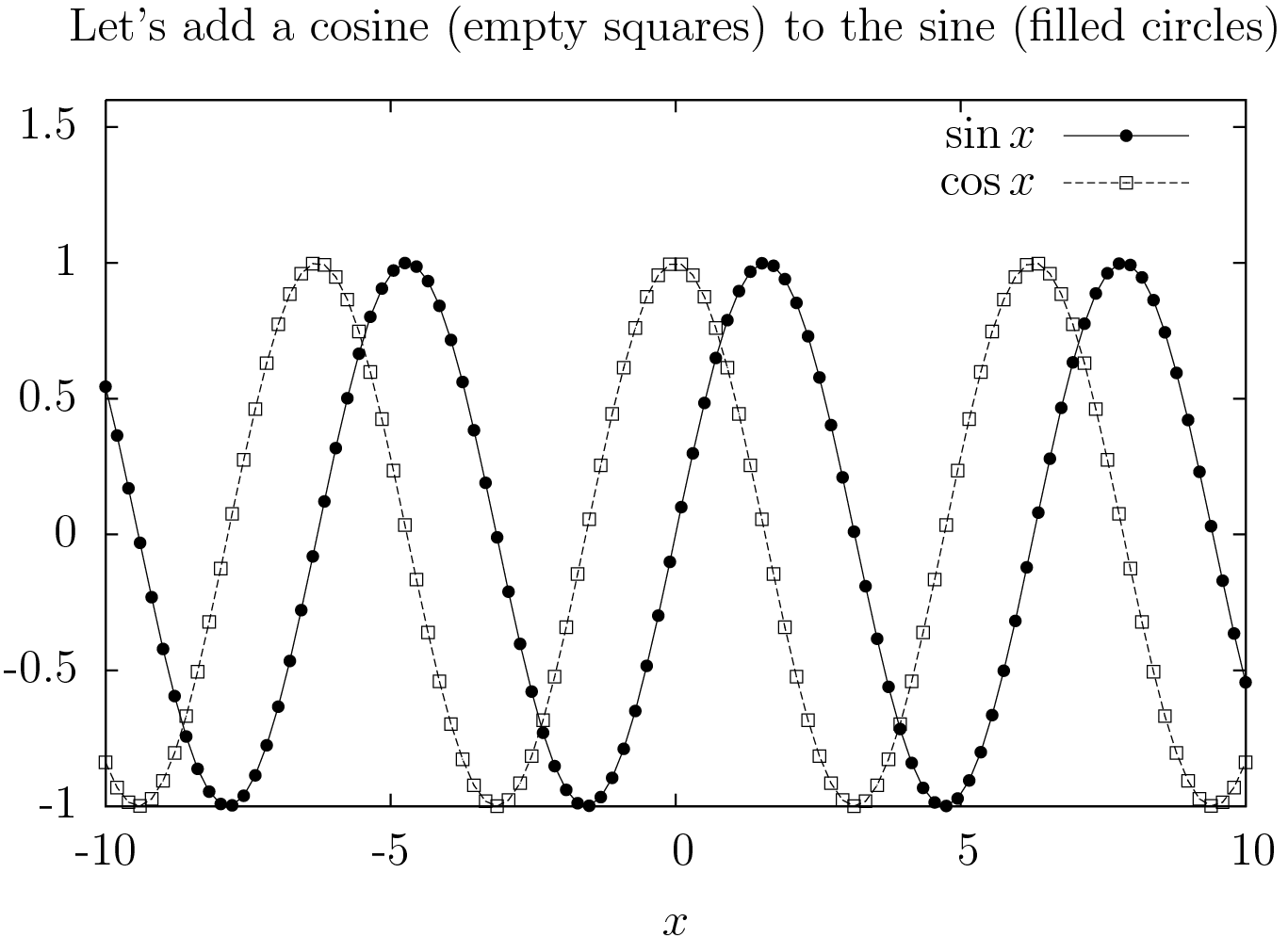
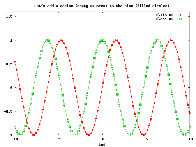
% A first simple gnuplot command
gps("plot sin(x) t '$\\sin x$' w lp pt 7;\
     set auto;\
     set yrange[-1:1.6];\
     set xlabel '$x$';\
     set title 'Let''s plot a sine with bullets (filled circles)'")
disp(["wait please " num2str(delay) " seconds..."]);fflush(stdout);pause(delay);
% Add a cosine
gps("replot cos(x) t '$\\cos x$' w lp pt 4;\
     set title 'Let''s add a cosine (empty squares) to the sine (filled circles)'")
% This makes the png figure you see on the webpage
gps("set terminal png transparent;set output 'demogps2d1.png';rep;set term x11")
% This makes the ps figure you see on the webpage
gps("ps","demogps2d1")
The Octave code above generates the following plot on the Gnuplot window.
The above plot produces, when exported through gps, the postscript file below:
Top
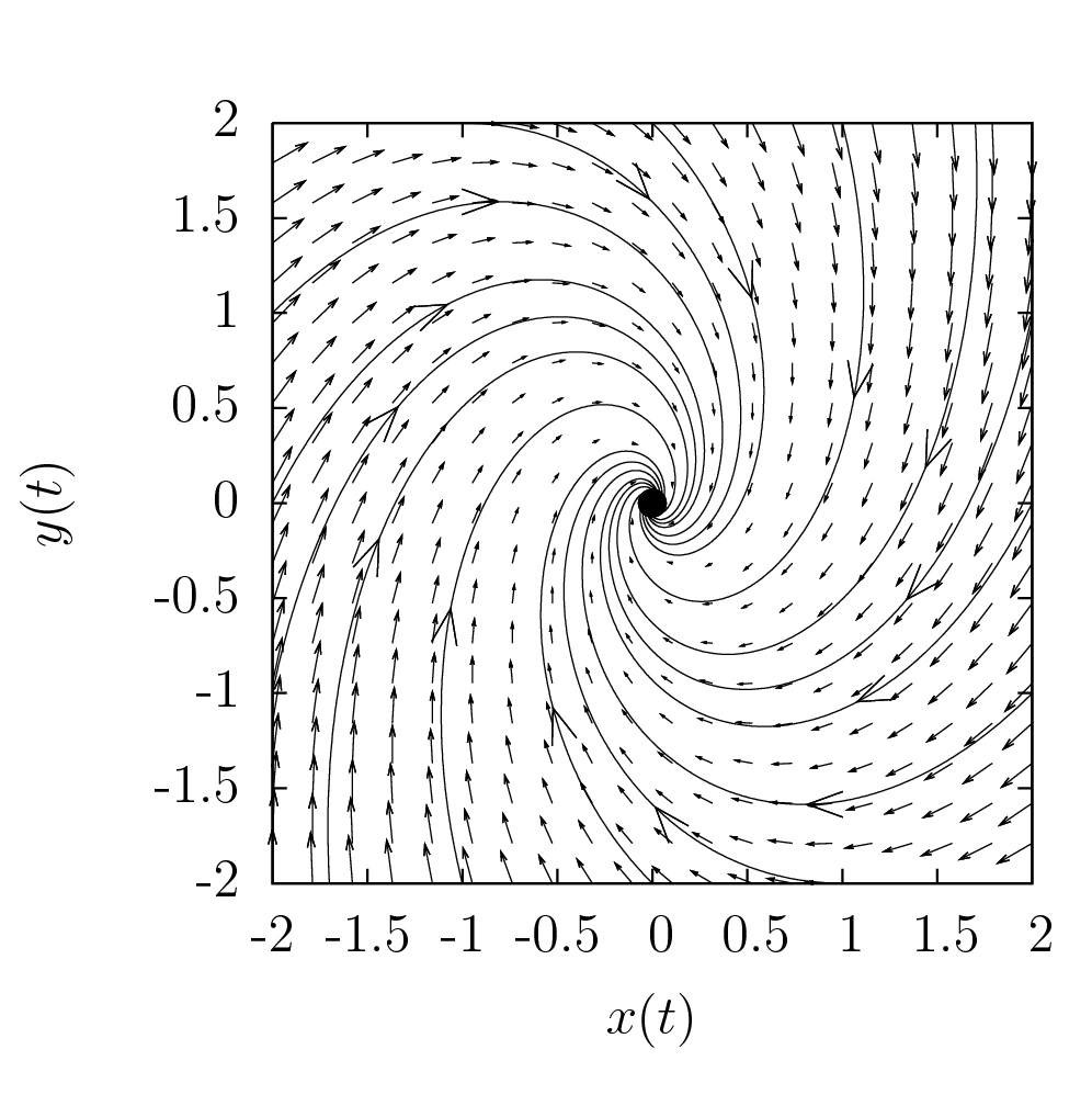
% Prepare the plot area
gps(["set size square;\
      set xrange[" num2str(xmin) ":" num2str(xmax) "];\
      set yrange[" num2str(ymin) ":" num2str(ymax) "];\
      unset key;\
      set xlabel '$x(t)$';\
      set ylabel '$y(t)$';\
      set title 'This is a stable spiral';\
      " ])

% This is to generate the spirals
for i=1:length(x0)
   % Solve the ode
   x =  lsode("dsys", x0(i,:), t)';
   if (i>1)
      pltoption="replot";
   else
      pltoption="plot";
   endif
   % Plot the current spiral
   gps(pltoption,[x(1,:)' x(2,:)'],"t '' w l 1")
   % This is for the arrow
   it=85;
   scale=0.05*max(abs(xmax-xmin),abs(ymax-ymin));
   % Plot the arrow for the current spiral
   gps(["set arrow from " num2str(x(1,it)) "," num2str(x(2,it)) " to "\
             num2str(x(1,it+1)) "," num2str(x(2,it+1)) " size " num2str(scale)\
	     ", 20 lt 1"]);
end
% Add a filled circle in the origin
gps("replot",[0 0],"t '' w p pt 7 ps 2")
% Generate vecotr field
yn=xn=20;
[X,Y]=meshgrid(linspace(xmin,xmax,xn),linspace(ymin,ymax,yn));
dX=aa(1)*X + aa(2)*Y;
dY=aa(3)*X + aa(4)*Y;
% Normalize vectors.
L = 7*sqrt(dX.^2 + dY.^2);
% To avoid normalization leave the next line uncommented, otherwise comment it
L = .5*max(max(L))*ones(size(dX));
% Finally, plot. Note that this single line is equivalent to quiver
gps("replot",[X(:) Y(:) (dX./L)(:) (dY./L)(:)],"w vectors lt 1")
% Remove the title just for the plots
gps("set title ''")
% This makes the ps figure you see on the webpage
gps("psbk","demogps2d2")
% This makes the png figure you see on the webpage
gps("set terminal png transparent;set output 'demogps2d2.png';rep;set term x11")
The Octave code above generates the following plot on the Gnuplot window.
The above plot produces, when exported through gps, the postscript file below:
Top
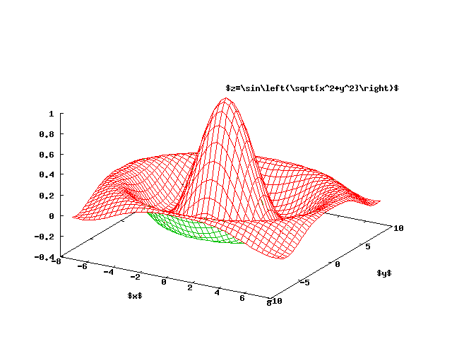
% Number of points in x and y
n=41;
% Prepare data for plot
tx = ty = linspace (-8, 8, n)';
[xx, yy] = meshgrid (tx, ty);
r = sqrt (xx .^ 2 + yy .^ 2) + eps;
tz = sin (r) ./ r;
% Plot using surface and various gnuplot stuff
gps("splots",tx,ty,tz,"w l t '';\
        set surface;\
        set hidden3d;\
        set ticslevel 0;\
        set xlabel '$x$';\
        set ylabel '$y$';\
        set label '$z=\\sin\\left(\\sqrt{x^2+y^2}\\right)$' at  0,0,1.1;\
        set title 'This is the famous sombrero';\
        ")
% Remove the title just for the plots
gps("set title ''")
% This makes the ps figure you see on the webpage
gps("psbk3d","demogps3d1")
% This makes the png figure you see on the webpage
gps("set terminal png transparent;set output 'demogps3d1.png';rep;set term x11")
The Octave code above generates the following plot on the Gnuplot window.
The above plot produces, when exported through gps, the postscript file below:
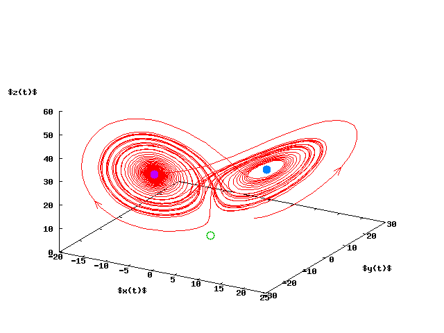
Top
% Solve the ode
x =  lsode("dsys", x0(i,:), t');
% Plot the solution as a single line in 3D
gps("splot",[x(:,1) x(:,2) x(:,3)],"t '' w l 1")
% Plot an arrow
it=10;
gps(["set arrow from " num2str(x(it,1)) "," num2str(x(it,2)) \
     "," num2str(x(it,3)) " to "\
    num2str(x(it+1,1)) "," num2str(x(it+1,2)) "," \
    num2str(x(it+1,3))  " size graph 0.02, 20 lt 1"]);
% Plot another one
it=3030;
gps(["set arrow from " num2str(x(it,1)) "," num2str(x(it,2)) \
     "," num2str(x(it,3)) " to "\
    num2str(x(it+1,1)) "," num2str(x(it+1,2)) "," \
    num2str(x(it+1,3))  " size graph 0.02, 20 lt 1"]);
% Set the axis stuff
gps(["set auto;\
      unset key;\
      set xlabel '$x(t)$';\
      set ylabel '$y(t)$';\
      set zlabel '$z(t)$' offset graph 0.05,0.05,.55;\
      set ticslevel 0;\
      set title 'This is the famous Lorenz attractor';\
      " ])
% Plot the stable and unstable equilibria
gps("replot",[0 0 0],"t '' w p pt 6 ps 2",\
            [sqrt(aa(2)*aa(3)-aa(3)) sqrt(aa(2)-1)*sqrt(aa(3)) aa(2)-1],\
	           "t '' w p pt 7 ps 2",\
            [-sqrt(aa(2)*aa(3)-aa(3)) -sqrt(aa(2)-1)*sqrt(aa(3)) aa(2)-1],\
	           "t '' w p pt 7 ps 2")
% Remove the title just for the plots
gps("set title ''")
% This makes the png figure you see on the webpage
gps("psbk3d","demogps3d2")
% This makes the png figure you see on the webpage
gps("set terminal png transparent;set output 'demogps3d2.png';rep;set term x11")
The Octave code above generates the following plot on the Gnuplot window.
The above plot produces, when exported through gps, the postscript file below:
Top